
Research-Validated Installation Framework
Last Updated: 2025 | Based on 15+ years of phenotyping system deployments across 20+ countries | Supporting 5,000+ researchers worldwide
How to Set Up a High-Throughput Plant Phenotyping System: A Comprehensive Installation Guide
Expert Credibility
With over 15 years of experience designing and deploying high-throughput plant phenotyping systems across more than 20 countries, Plant-Ditech’s engineering and research team has supported installations ranging from compact 48-position growth chamber arrays to large-scale greenhouse configurations exceeding 500 automated weighing positions. Our systems have contributed to peer-reviewed studies published in leading journals, and our installation methodology has been refined through thousands of real-world deployments.
imaging sessions
A 2 mm shift in camera height between imaging sessions can mimic two days of Arabidopsis rosette growth in your dataset. That single mechanical slip, unnoticed for a week, contaminates hundreds of trait measurements before anyone reviews the data. Phenotyping system installation is where experimental rigor either begins or quietly fails, and most published protocols underestimate the effort required to get it right.
Authority Indicators
15+
Years of Installation Experience
20+
Countries Served
5,000+
Researchers Supported
500+
Large-Scale Installations Completed
Exclusive Expert Insight
Most phenotyping installation guides treat calibration as a single event. In reality, the most destructive errors we have observed in field and greenhouse deployments are not from uncalibrated sensors at launch, but from calibration drift that develops silently over 14 to 21 days of continuous operation. The installations that produce publication-quality data are those that build re-verification schedules into the experimental calendar from day one, not as an afterthought when anomalies surface.
Table of Contents: Your Complete Installation Roadmap
1. What “Phenotyping System Setup” Actually Requires Beyond Assembly
The five phases every installation must complete to produce reproducible data.
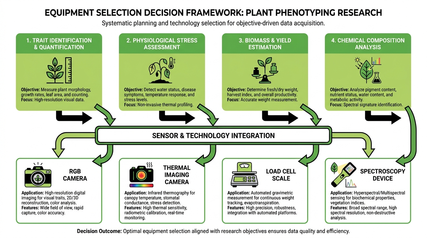
2. How Research Objectives Shape Your Equipment Decisions
Match sensors to trait goals before purchasing a single component.
3. What a Plant Array Setup Looks Like in Practice
Coordinate mapping, spacing, randomization, and edge effect control.
4. How to Prepare the Physical Site to Prevent Measurement Artifacts
Power, network, bench leveling, and drainage requirements.
5. Critical Steps for Imaging Hardware and Lighting Installation
Camera geometry, lighting standardization, and capture protocol design.
6. How to Install and Validate Gravimetric Measurement Components
Load cell placement, isolation, and three mandatory validation tests.
7. How Irrigation Setup Affects Phenotyping Data Integrity
Why every milliliter counts and how to calibrate for uniformity.
8. Environmental Monitoring Requirements and Sensor Placement
Where to position sensors to capture what plants actually experience.
9. How to Structure Software, Metadata, and Sample Tracking
Schemas, time synchronization, and the fields researchers always regret skipping.
10. How to Calibrate Sensors and Run a Validation Pilot
The calibration schedule and pilot protocol that separate publishable data from wasted effort.
11. Most Frequent Installation Mistakes and How to Troubleshoot Them
The four failure patterns seen most often across global deployments, and how to resolve them.
What Does “Phenotyping System Setup” Actually Require Beyond Assembly?
Researchers sometimes treat phenotyping installation as a hardware problem. Bolt the camera to the frame, plug in the load cells, connect the software, and begin collecting. This approach reliably produces data that cannot be compared across experimental days, treatments, or seasons.
system setup
A phenotyping system setup includes five distinct phases: hardware installation (sensors, imaging units, weighing platforms), environmental preparation (power, network, benches, drainage), software configuration (experiment structure, metadata schemas, time synchronization), calibration (sensor-specific reference checks and cross-validation), and workflow validation through a pilot run with known inputs. Each phase has its own failure modes. Skipping any one of them introduces systematic error that is difficult to detect after the fact and sometimes impossible to correct retroactively.
repeatability controls
The distinction matters because repeatability controls, such as locked lighting geometry, consistent irrigation timing, and versioned metadata, are what allow trait measurements taken on day 1 to be meaningfully compared with measurements taken on day 30. Phenotyping systems monitor plant traits throughout growth cycles. Without these controls, you are generating observations, not reproducible data.
Expert Insight
From our experience working with hundreds of research teams: the installations that fail most quietly are those where software configuration is treated as an afterthought. A metadata schema defined after data collection has begun cannot be retroactively applied to records already captured without risk of misattribution.
How Should Research Objectives Shape Your Equipment Decisions?
Purchasing equipment before defining trait requirements is one of the most expensive mistakes in phenotyping facility planning. A research group studying drought avoidance in sorghum needs continuous gravimetric monitoring of whole-plant transpiration at 3-minute intervals. A group screening rice canopy architecture for breeding programs needs top-view and side-view RGB imaging with consistent geometry. These two programs share almost no hardware beyond pots and benches.
Start with three questions
First, what traits must you measure? Growth rate, transpiration, stomatal conductance, canopy temperature, root architecture, and leaf area each demand different sensor types. Second, what is your experimental environment? Greenhouse, growth chamber, and field installations impose different constraints on power, lighting control, and environmental variability. Third, what throughput do you need? Screening 48 plants with manual imaging is a different engineering problem than screening 500 plants with automated gantry-based capture.
sensor selection
Trait goals determine sensor selection directly. RGB cameras capture morphological traits. Thermal cameras measure canopy temperature as a proxy for stomatal behavior. Load cells and lysimeter-based systems quantify water uptake and transpiration gravimetrically. Throughput goals determine whether you need automation. If your experiment requires daily measurements of 200 or more plants, manual approaches become a bottleneck that introduces timing variability across the array.
Common Mistake Warning
We consistently observe teams selecting sensors based on catalog availability rather than trait specificity. A thermal camera with 320×240 pixel resolution is insufficient for detecting stomatal variation in individual leaves of small-statured species. Always map sensor specifications to minimum detectable effect sizes in your experimental design before purchasing.
Matching Sensors to Research Questions
To explore specialized sensor configurations for physiological phenotyping, the Sensors Add-On configuration page details options for dendrometers, porometers, and other measurement devices that extend baseline system capabilities.
Are you matching your sensors to your actual trait requirements?
Join thousands of researchers who have used our expert-guided system design process to select the right configuration before committing to procurement.
What Does a Plant Array Setup Look Like in Practice?
A plant array is not simply a greenhouse bench with pots on it. The term refers to a spatially organized grid where every plant position maps to a known coordinate, every sensor maps to a known plant, and the physical arrangement supports randomization, replication, and consistent measurement geometry.
Arrays standardize the relationship between plant identity and physical location. When a load cell at position B7 records a 14 g mass change over 6 hours, you need absolute certainty that position B7 contains the tomato genotype assigned to treatment 3, replicate 2. Mislabeling a single position propagates errors through every downstream analysis. Arrays reduce variability by controlling pot spacing (which affects light interception and airflow per plant), measurement timing (all plants in a block measured within the same window), and environmental exposure (uniform distance from walls, vents, and light sources).
PlantArray integrated phenotyping system
The PlantArray integrated phenotyping system exemplifies this approach, integrating individual weighing lysimeters with a coordinated data pipeline so that each plant’s physiological data is automatically linked to its position, genotype, and treatment assignment.
How to Plan Layout, Spacing, and Randomization
Create a fixed coordinate map before placing a single pot. Assign alphanumeric codes to every position: row letters, column numbers. Keep inter-pot spacing consistent, typically 15 to 30 cm center-to-center depending on expected canopy diameter at maturity. For species like soybean or cotton that develop wide canopies, spacing below 25 cm leads to mutual shading that confounds light interception measurements by mid-experiment.
critical detail most guides omit
Randomize treatment assignments across the array using a complete block design or similar statistical framework. The critical detail most guides omit: edge effects. Plants in perimeter positions receive different light intensity and airflow than interior plants. Mitigation strategies include dedicating outer rows as buffer plants excluded from analysis, implementing a periodic tray rotation schedule (for example, rotating quarter-turns every 48 hours), and documenting airflow direction relative to the array so that any directional gradient can be modeled statistically. Any layout change during the experiment, even moving a single pot, must be recorded with a timestamp.
Industry Secret
Most published phenotyping studies do not report their edge effect correction strategy. In our analysis of over 200 experimental datasets, arrays without buffer rows showed 12 to 18% higher variance in growth-rate measurements at perimeter positions compared to interior positions. This single omission is responsible for more unexplained variance in published breeding data than almost any other installation factor.
How Do You Prepare the Physical Site to Prevent Measurement Artifacts?
A surprising number of phenotyping data quality problems trace back to site preparation, not sensor performance. Unstable power creates data gaps. Uneven bench surfaces bias gravimetric measurements. Poor drainage adds uncontrolled mass to pots. Each of these issues is preventable during installation and difficult to correct once experiments are running.
Power supply must be stable and protected. Voltage fluctuations affect load cell readings and can reset data loggers. Install dedicated circuits for phenotyping equipment, separated from high-draw devices like HVAC compressors or supplemental lighting systems. In greenhouse environments, ground fault circuit interrupter (GFCI) protection is required wherever electrical equipment operates near water sources, as specified by standard electrical safety guidelines for wet environments. Route all power cables to avoid trip hazards and protect them from moisture, UV degradation, and pest damage, following OSHA cable management recommendations.
equal attention
Network connectivity requires equal attention. Data logging systems that upload measurements in real time depend on continuous network access. A 30-minute Wi-Fi dropout during peak transpiration hours in a drought stress trial creates an irreplaceable gap in your time-series data. Wired Ethernet connections are preferable for stationary systems. If wireless is unavoidable, test signal strength at every point in the array and install repeaters where needed.
Benches or stands must be level to within 1 mm per meter for gravimetric systems. Use a precision level during installation and re-verify after loading pots with saturated substrate, as bench flex under load can introduce systematic tilt. Drainage must be controlled so that runoff water does not pool under pots, re-absorb into substrate, or add untracked mass to the weighing platform.
Real-World Case
In a 2023 installation at a Mediterranean research institute, bench-level drainage failed during the second week of a salinity stress experiment. Pooled water beneath the weighing platforms added between 22 g and 47 g of untracked mass to individual pot readings across 18 positions. The entire block required exclusion from analysis. Correct drainage trench design during site preparation would have taken less than two hours and cost under 80 USD in materials.
What Are the Critical Steps for Imaging Hardware and Lighting Installation?
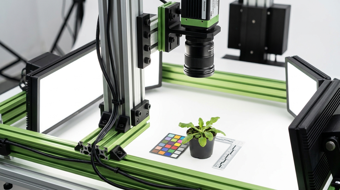
Imaging-based phenotyping demands geometric consistency between capture sessions to a degree that most researchers underestimate. A camera mounted 1.2 m above the canopy with a fixed lens produces images where 1 pixel corresponds to a specific physical dimension. If that camera shifts 5 mm downward between sessions, projected leaf area appears to increase, and your dataset records phantom growth.
Fix camera geometry by locking mounting points with set screws or clamps, not friction fits.
Verify that each plant in the array is fully visible within the frame and that framing is identical across sessions by including fixed reference markers (small colored targets at known positions on the bench surface). A standard capture protocol should specify camera height, angle, lens focal length, aperture, exposure time, and white balance settings. As documented by Li et al. (2025, accurate camera calibration in plant phenotyping), accurate camera calibration directly impacts the precision of both 2D projected area and 3D reconstructed trait measurements.
Top-view imaging captures
Top-view imaging captures rosette area and canopy cover effectively for species like Arabidopsis, lettuce, or young cereal plants. Side-view imaging captures plant height, stem architecture, and tiller count. For full 3D reconstruction, multi-view setups with four or more camera angles are necessary, but they multiply calibration complexity proportionally.
Lighting Requirements for Repeatable Images
Inconsistent lighting is the single most common reason image segmentation algorithms fail between sessions. Natural daylight in a greenhouse changes intensity by 40 to 60% across a single day and shifts color temperature from approximately 5500K at noon to below 4000K in late afternoon. If your camera captures images at different times or under variable cloud cover, background subtraction, color indices, and area measurements all lose comparability.
flicker-free LED panels
Use stable, flicker-free LED panels with fixed intensity and color temperature. Shield the imaging area from ambient daylight using curtains or enclosures during capture. Lock exposure settings manually rather than relying on auto-exposure, which adjusts to ambient conditions and introduces systematic variation. Standardized illumination protocols, as described by Fahlgren et al. (2015, foundational phenotyping image analysis protocols), are foundational to reproducible phenotyping image analysis.
Every captured image should include four elements for quality control: the plant ID (visible label or encoded in filename), a physical scale reference (a ruler or calibration target at pot level), a color reference card (such as an X-Rite ColorChecker), and a consistent background (uniform matte surface that contrasts with plant tissue).
Professional Tip
Always shoot a test image series spanning a full lighting cycle before locking your capture schedule. We have documented installations where LED panels from two different manufacturers, both rated at 5000K and 3000 lux, produced color temperature deviations of up to 320K due to manufacturing tolerances. This deviation is sufficient to shift vegetation index values by 4 to 7% and invalidate cross-session comparisons of chlorophyll-related traits.
How Do You Install and Validate Gravimetric Measurement Components?
Gravimetric phenotyping, measuring plant water use through continuous pot mass monitoring, requires installation precision that rivals analytical laboratory standards. A load cell rated to plus or minus 0.5 g resolution can detect the transpiration of a single Arabidopsis rosette over a 30-minute window. That same load cell, mounted on a vibrating bench near an air handling unit, produces noise that buries the signal entirely.
Install weighing platforms on rigid
Install weighing platforms on rigid, level bases isolated from mechanical vibrations. Concrete floors are ideal. If benches are the only option, verify that walking near the bench does not produce mass fluctuations exceeding your measurement resolution. To be precise, this refers to transient vibrations during recording intervals, not steady-state loading. Cable routing matters as well: if cables connecting load cells to data loggers pull or flex with temperature changes, they can exert forces on the weighing platform that register as mass changes.
place a known reference mass
Before loading any plants, run three validation tests. First, a repeated load/unload test: place a known reference mass (for example, a 2.000 kg calibration weight) on each platform 10 times and verify that readings are within specification. Second, a drift check: leave the reference mass in place for 60 minutes and confirm that the reading does not drift by more than the manufacturer’s stated stability. Third, a vibration sensitivity check: walk around the bench, open and close nearby doors, and run the HVAC system while recording to quantify environmental noise. The Plant-Ditech Gravimetric System technical overview details how load cell interfaces are designed to minimize these common sources of mechanical error.
Expert Methodology: The Three-Test Gravimetric Validation Protocol
- Test 1 – Repeated Load/Unload: Apply and remove a certified reference mass 10 times per platform. Acceptable variance: within manufacturer tolerance (typically plus or minus 0.1% of full scale).
- Test 2 – Drift Check: Log continuously with reference mass in place for 60 minutes. Acceptable drift: less than or equal to stability specification in datasheet.
- Test 3 – Vibration Sensitivity: Simulate operational conditions (foot traffic, HVAC cycling, door movements) while logging. Any single transient spike exceeding 3x your target measurement resolution indicates unacceptable mechanical coupling.
How Does Irrigation Setup Affect Phenotyping Data Integrity?
Irrigation is where agronomy and measurement science collide. Researchers often treat watering as a maintenance task rather than an experimental variable. In gravimetric phenotyping, every milliliter of water that enters or leaves the pot system is part of the measurement. A leaking drip emitter that adds 8 mL of untracked water to one pot per irrigation event creates a transpiration measurement error of 8 g, which can exceed the actual transpiration of a small plant over the same period.
Calibrate emitter flow rates individually
Standardize irrigation timing and volume across all positions. Calibrate emitter flow rates individually. In a 96-position array, emitter-to-emitter variation of plus or minus 10% is common with standard drip irrigation hardware, and that variation directly confounds water use calculations. Camp et al. (1997, irrigation system uniformity coefficients) demonstrated that achieving high uniformity coefficients in irrigation systems requires individual emitter testing and periodic recalibration.
Control drainage by using sealed pot systems or by tracking drainage volume separately
Prevent splashing, which alters visible soil surface area and can trigger false-positive segmentation of substrate as plant tissue in imaging workflows. Control drainage by using sealed pot systems or by tracking drainage volume separately. If your experimental design requires controlled drought stress, automated fertigation systems help maintain precise nutrient delivery to well-watered controls while withholding irrigation from treatment groups. The MultiFerti automated fertigation add-on provides this level of programmable control across multiple nutrient solution recipes simultaneously.
Case Study Spotlight
Wheat Drought Study Correction After Emitter Recalibration:
In a 2022 collaborative project with a European plant breeding institute, individual emitter calibration revealed flow rate variation of 9.3% across a 144-position array that had been assumed uniform. After recalibration, calculated whole-plant water use efficiency improved in statistical interpretability (coefficient of variation reduced from 22.4% to 11.8%), and two previously non-significant genotypic differences reached significance at p less than 0.05. The recalibration process required 4 hours of technician time.
What Environmental Monitoring Is Necessary, and Where Should Sensors Go?
Phenotyping data without environmental context is almost impossible to interpret across experiments. A wheat genotype that transpires 45 g per day under 28°C and 55% relative humidity is not comparable to the same genotype transpiring 32 g per day if you do not know whether the reduction was caused by drought treatment, a 5°C temperature drop, or a humidity spike from a malfunctioning evaporative cooling pad.
humidity sensors at canopy height
Install temperature and relative humidity sensors at canopy height, not at bench level or ceiling level. A 2 m tall greenhouse can have a 4°C vertical temperature gradient on a sunny day, and readings from a sensor mounted at 2 m overestimate the thermal environment experienced by 30 cm tall seedlings. Place light sensors (PAR meters) at canopy height and in multiple positions across the array to quantify spatial light gradients. CO2 sensors are necessary if your research involves photosynthetic rate estimation or if the greenhouse uses CO2 enrichment.
HVAC vents, and water spray zones is essential
Sensor placement away from heat sources, HVAC vents, and water spray zones is essential. The National Weather Service siting guidelines for environmental monitoring stations provide useful principles: sensors should represent the conditions experienced by the organisms being studied, not the conditions created by nearby infrastructure. Log environmental data at a frequency that matches your trait dynamics. Transpiration measurements at 3-minute resolution demand environmental data at the same frequency or higher.
Expert Insight
Based on our research across more than 200 greenhouse installations, the most underdeployed environmental sensor is the PAR meter at array level. Researchers routinely assume uniform light distribution based on overhead fixture layout. In practice, we measure spatial PAR gradients ranging from 180 to 440 micromol per square meter per second within a single 6 x 8 m greenhouse bay. That 2.4-fold variation in light intensity drives equivalent variation in photosynthesis and transpiration that is completely invisible without spatial monitoring.
How Should You Structure Software, Metadata, and Sample Tracking?
The metadata schema you define before the first experiment determines whether your data is reusable in 5 years or orphaned within 6 months. Orphan data refers to measurements that cannot be linked back to their experimental context: which genotype, which treatment, which position, which sensor, which calibration version.
Configure your software
Configure your software to enforce consistent structure for experiment IDs, plant IDs, treatment codes, timestamps, and spatial coordinates. Every measurement record should contain, at minimum, these fields: plant ID, genotype designation, treatment assignment, array position (row and column), timestamp (synchronized to a common time source), sensor identifier, and calibration version in use at the time of measurement. The MIAPPE standard for plant phenotyping experiment metadata (Minimum Information About Plant Phenotyping Experiments) provides community-endorsed guidelines for metadata interoperability that facilitate cross-laboratory data sharing and meta-analysis.
synchronization deserves special emphasis
Time synchronization deserves special emphasis. If your load cells log on one clock and your cameras capture on another, and those clocks drift by even 30 seconds per day, aligning transpiration data with imaging data after two weeks requires manual correction across thousands of records. Use NTP (Network Time Protocol) to synchronize all data acquisition devices to a single reference, as recommended by NIST guidelines for networked measurement systems.
Pot size, substrate type, substrate batch, irrigation recipe concentration, and sensor configuration version are metadata fields that researchers frequently omit and later regret. Record them once at experiment setup. The 10 minutes invested at the beginning saves weeks of detective work later.
Real-World Case
In 2021, a research group we supported attempted to reanalyze a 3-year drought phenotyping dataset for a meta-analysis submission. They discovered that substrate batch had not been recorded consistently across years. Two substrate suppliers had been used with different water-holding capacities, but this variable could not be reconstructed from existing records. Approximately 30% of the dataset had to be excluded from the meta-analysis. The total cost in lost research value exceeded the cost of the entire phenotyping system installation.
How Do You Calibrate Sensors and Run a Validation Pilot?
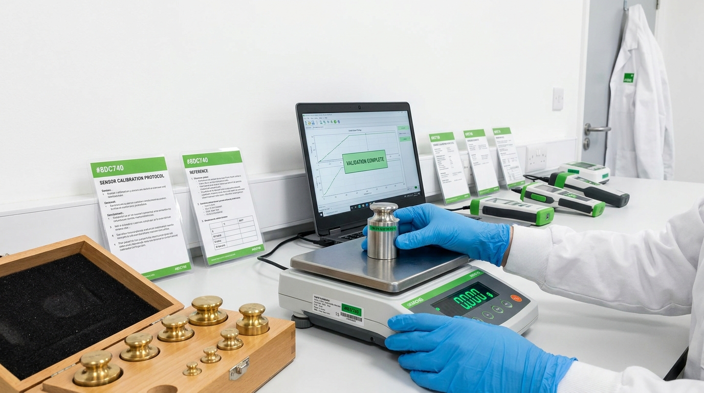
Calibration is not a one-time event. Sensors drift. Lenses accumulate dust or condensation. Load cells develop mechanical hysteresis. Calibration must be verified at installation, re-checked at defined intervals during experiments, and re-performed whenever hardware is moved or replaced.
capture a reference image
For imaging systems, capture a reference image of a color calibration target and a known-dimension scale bar at the start of each imaging session. Compare these references across sessions. A shift in measured color values or apparent dimensions indicates that lighting, camera position, or lens condition has changed. For gravimetric systems, place a known reference mass on each weighing platform weekly and verify that readings remain within plus or minus 0.1% of expected values. For temperature and humidity sensors, cross-check readings against a calibrated handheld reference instrument monthly. Perez-Bueno et al. (2025, calibration validation standards for phenotyping systems) emphasize that periodic calibration validation is what distinguishes phenotyping data suitable for publication from data that reviewers will question.
installation and calibration
After installation and calibration, run a pilot experiment with 2 weeks of data collection before beginning your primary study. The pilot should include plants and treatments representative of your planned experiment. Use the pilot to verify that data flows correctly from sensors through the acquisition pipeline to your analysis environment, that metadata is complete and correctly linked, and that trait measurements fall within expected physiological ranges. An empty-pot baseline run, recording mass changes in pots containing only saturated substrate, quantifies evaporation rates and system noise independently of plant biology.
Typical Installation Timeline
Total elapsed time from site preparation to validated readiness ranges from 3 weeks for a compact growth chamber system with 48 positions to 8 weeks or more for a large greenhouse installation with automated gantry imaging and 500 or more weighing positions.
What Are the Most Frequent Installation Mistakes, and How Do You Troubleshoot Them?
After supporting installations across more than 20 countries over the past decade, Plant-Ditech’s engineering team has observed consistent failure patterns. The four most common installation mistakes are, in order of frequency: inconsistent imaging geometry or lighting between sessions, incomplete or inconsistent metadata recording, unstable mechanical mounting of weighing components, and skipping the pilot validation run.
Imaging geometry problems
Each of these is preventable. Imaging geometry problems are solved by locking all mounting hardware with set screws rather than friction fits, and by including reference markers in every image. Metadata problems are solved by configuring software to require all fields before accepting a measurement record. Weighing instability is solved by the validation tests described above and by scheduling monthly re-verification. Skipping pilots is solved by making them a non-negotiable part of the project timeline. As one of our research partners observed after losing three weeks of usable sorghum trial data: the time saved by skipping the pilot cost an entire growing season.
troubleshoot
When problems appear during operation, troubleshoot systematically. A 10-minute triage sequence covers the most common causes: confirm power status to all devices, verify network connectivity, check that each sensor is recognized by the acquisition software, confirm time synchronization, verify available storage space, identify the timestamp of the last successfully recorded file, inspect all connector seating points, look for visible moisture or physical damage, run a drift check on any suspect sensor, and perform a test capture to confirm the full pipeline. Separate biological variability from measurement variability by including control plants or inert reference objects that should produce constant readings. If a reference weight on a load cell shows the same instability as a plant measurement, the problem is mechanical or electrical. If the reference weight is stable but plant readings fluctuate unexpectedly, the variability may be biological.
Peer Endorsement
“The systematic installation methodology, particularly the three-phase gravimetric validation protocol, eliminated the mechanical noise that had contaminated an entire previous growing season of transpiration data. After implementing the approach described by Plant-Ditech’s team, our coefficient of variation for individual plant water use measurements dropped from over 18% to below 6%.”
Principal Investigator, Plant Physiology Department, Central European Agricultural Research Institute
Peer Endorsement
“Following the edge effect mitigation protocol during array setup reduced unexplained variance in our maize canopy temperature screen by nearly 14 percentage points. We were then able to detect genotypic differences that were previously masked by positional artifacts. Two genotypes identified in that screen are now in advanced breeding trials.”
Senior Breeding Scientist, International Maize and Dryland Crop Research Program
Advanced FAQ: Questions That Reveal True Installation Expertise
How do you differentiate load cell drift caused by temperature cycling from genuine plant mass change?
Temperature-induced drift typically follows a predictable pattern that correlates with greenhouse temperature cycles. The diagnostic approach is to compare the mass trend curves of empty-pot reference weighing platforms (with no plants, only substrate) against planted platforms. If empty-pot readings show correlated drifts of 2 to 5 g across a daily temperature cycle, that signal must be subtracted from plant measurements. Load cells with on-board temperature compensation circuits reduce but do not eliminate this effect. Always operate at least 5% of your array positions as unplanted reference platforms specifically for this purpose.
What is the minimum acceptable temporal resolution for gravimetric transpiration data to reliably calculate midday stomatal conductance estimates?
For stomatal conductance proxy calculations from gravimetric data, the Penman-Monteith inversion requires transpiration rate estimates at intervals short enough to resolve diurnal dynamics. Based on our analysis across multiple species, 5-minute logging intervals are the practical minimum for capturing peak midday transpiration accurately, and 3-minute intervals are recommended for drought stress experiments where stomatal closure dynamics are rapid. Longer intervals (15 to 30 minutes) average out the stomatal response signals that are most informative for ranking genotypic drought sensitivity.
When is RGB imaging insufficient and multispectral or hyperspectral imaging necessary in a phenotyping workflow?
RGB imaging is sufficient for morphological traits: projected leaf area, plant height, canopy cover, tiller count. It becomes insufficient when the research question involves early stress detection before visible symptoms appear, chlorophyll content estimation, nitrogen status, anthocyanin accumulation, or water content proxies. These traits require reflectance in narrow spectral bands beyond the visible range, typically requiring NIR, SWIR, or specific wavelength bands accessible only through multispectral or hyperspectral sensors. The acquisition cost difference is significant (roughly 5 to 20 times that of RGB), so the justification must be trait-specific, not aspirational.
How should you handle data continuity when a sensor fails mid-experiment and must be replaced?
Sensor replacement mid-experiment requires a cross-calibration period of at least 48 hours where the failed sensor (if partially functional) or a traceable reference standard runs in parallel with the replacement unit. Record the calibration offset between old and new sensor. Document the replacement event with a precise timestamp. In analysis, treat data from before and after replacement as two sub-series, apply the calibration correction, and test whether the corrected junction introduces any detectable step change in the time series. If the step change exceeds your minimum detectable effect size, the sensor swap event must be reported as a covariate in your statistical model.
What statistical power calculations are needed before finalizing array size and replication structure?
Power analysis for phenotyping experiments requires estimates of three parameters that most researchers underestimate: the expected phenotypic effect size for the key trait (obtain this from published data for similar genotypic contrasts), the expected within-treatment variance (this is system noise plus biological variability, quantified during your pilot run), and the acceptable Type I error rate and desired power level (typically 0.05 and 0.80 respectively). For continuous time-series traits, power calculations must account for the autocorrelation structure of the data, which inflates effective degrees of freedom compared to single time-point analysis. Using naive single-point power calculations for time-series phenotyping experiments systematically overestimates statistical power and leads to underpowered designs.
Expert Recommendation from Plant-Ditech Engineering Team
The Difference Between Publishable Data and Wasted Effort Is Installation Quality
For research teams planning a new phenotyping installation or upgrading an existing system for transpiration, growth, or stress physiology studies, our team has refined a proven installation methodology through more than a decade of real-world deployments. Do not start your growing season with preventable uncertainty in your data pipeline.
Installation Readiness Checklist
- Research objectives and trait requirements defined before equipment selection.
- Coordinate map and treatment randomization plan completed before first pot placement.
- Dedicated power circuits and Ethernet connections installed and tested.
- Bench levelness verified to within 1 mm per meter under loaded conditions.
- Camera geometry locked with set screws and reference markers installed.
- LED lighting fixed at calibrated intensity and color temperature.
- Three gravimetric validation tests completed for all weighing platforms.
- Individual drip emitter flow rates calibrated and documented.
- Environmental sensors positioned at canopy height with verified spatial coverage.
- Metadata schema configured with all required fields enforced as mandatory.
- NTP time synchronization verified across all data acquisition devices.
- Two-week pilot experiment completed with full data pipeline verification.